Measures of central tendency (mean, median, mode, etc.) are some of the first concepts we learn in any basic statistics course. Such concepts are illustrated with several examples, such as: the mean height of the students in the class (or more sensitive information such as age or weight), or the mean/median salary of a company. It is essential to understand these concepts to better understand the world around us. In this post, however, the goal is not to explain neither the concepts, nor why they are important, but to answer the question: what does it have to do with computer science?
A straightforward application is to compute the mean execution time for a given algorithm. Which might help understanding asymptotic notation (e.g. Big O, O(1), O(N), O(NlogN)). Don’t worry if you have no idea what asymptotic notation is. I’d like to focus on another application: image processing.
Digital images
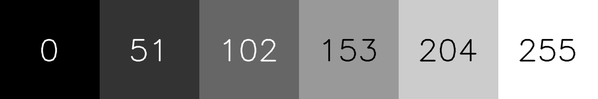
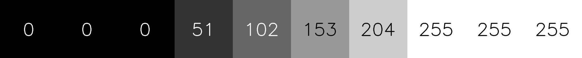
Before talking about image processing, let’s review what a digital image is. The most common way to represent an image in a computer is with a table, or matrix, of pixels. A pixel is the representation of a color, in a color image, or intensity, in a grayscale image. We will work with grayscale images for simplicity. Most grayscale images have 256 shades (no, not 50), or levels, varying from black (0) to white (255).
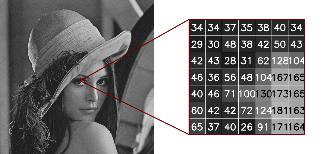
A grayscale image is just a table with numbers between 0 and 255:
Using means with images
Back to the measures of central tendency. As the image is just a table of numbers, we can compute its mean. For example, the mean of the image above is 91.52. It doesn’t say much, right? Let’s consider a single row instead:
Replacing each pixel by the mean of its neighbors (the pixels to the right and to the left, when they exist) with its own value, we have:
In this case, the mean smoothed the difference between adjacent pixels! Visually, the borders are smoothed and the whole image is blurred. Let’s see what happens when we consider 5 pixels for the mean (2 pixels to the left, 2 pixels to the right, and the pixel itself):
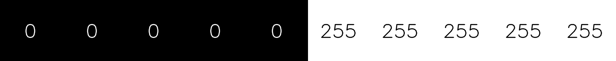
The process of image acquisition and storage isn’t perfect. Thus it’s common to have noise in the image. Let’s consider a simple case: a row of black pixels. We’ll add random noise: one of the pixels that should be black was registered as white.

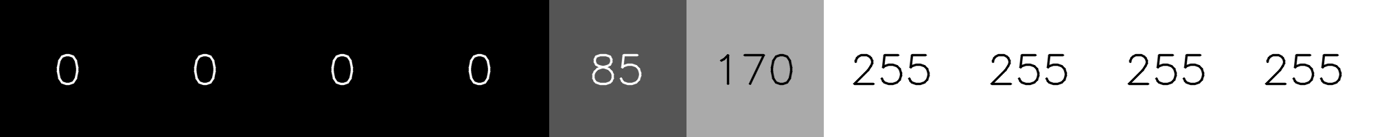
Let’s repeat the process of computing the mean of the 5 neighboring pixels:

As most of the pixels have the same intensity, the mean tends to get close their value. In this case, black. With this the white pixel turns darker. In other words, this process can be used to reduce the noise in an image. A collateral effect is the spreading of the noise to it’s neighbors, initially with the right color. This process of replacing a pixel by its neighbors mean value is known as mean filter or average filter.
Let’s add an extra dimension. We will now compute the mean using all the neighbors of a pixel. In other words, we will use not only the pixels to the right and left, but also the pixels above, below and at the diagonals.
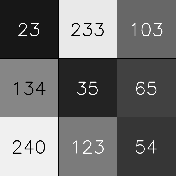
In the image above, the pixel 35 will be replaced by the mean value of its neighbors: (23 + 233 + 103 + 134 + 35 + 65 + 240 + 123 + 54) / 9 = 112.22. The observed effect will be the same we obtained for the single row. Now, let’s return to the original image and add some random noise (black and white pixels in random positions - also known as salt and pepper noise).

When we apply the mean filter using the 8 neighbors and the pixel itself we obtain the following result:

The set of pixels used to compute the mean is called window. The number of pixels in the window can be larger than 9. There are no limits for neither the size or shape of the window. The following image shows the application of a mean filter with 49 pixels in the window (a 7 x 7 pixels square).

In the extreme case we can use a very large window (larger than the image itself). In this case, each pixel will be replaced by the average of all the pixels in the image, in our example, 91.67. The result will be this image with a single grayscale intensity:

Medians and images
What would happend if we simply replace the mean by the median? Let’s initially consider a property of medians. The median of the set {0, 1, 100} is 1. It doesn’t matter how large or small the first and last numbers are. Likewise, the number 255 doesn’t affect the computation of the median of {0, 0, 0, 0, 255}, which will still be 0, no matter what we use instead of 255. This is not true for the mean. In the example of the row with one white pixel, the result of a median filter using a window of size 5 (two pixels to the left and two to the right) would be:

Let’s see what happens when the row is half black and half white:

This example shows an interesting property of median filters. While a mean filter blurs the whole image, smoothing the borders, a median filter preserves borders. Let’s see what happens when we apply the median filter to the noisy image (using a window of 3 x 3 pixels):

A disadvantage of using median filters instead of mean filters is its higher computational complexity. While the computation of the mean is linear (O(N)), where N is the number of pixels (we just have to sum all values and divide by N), the computation of the median takes O(NlogN) (we have to sort the pixel values to return the central one).
Another way to understand the effect of mean filters on images uses the concept of Fourier transform. I find this explanation particularly beautiful, but let’s leave it for a future post.